We measure the overlap between \(f\) and \(g\) when one function is "flipped" and shifted by \(x\).
Example (Dice - Not a Good Example)
Assume there are two 6-face dices. We want to know the probability of the sum of two dices equals to 4.
Define \(f(x) = \text{probability of getting x on dice 1}\), \(g(x) = \text{probability of getting x on dice 2}\). The probability of getting a sum of 4 is:
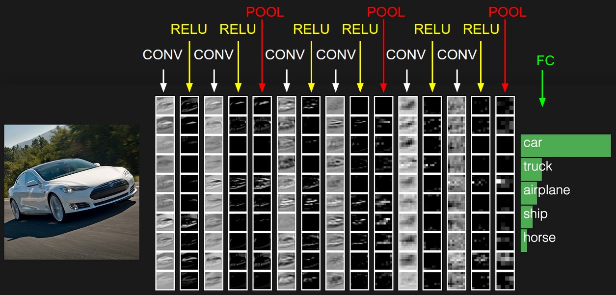
We use three main types of layers to build ConvNet architectures: Convolutional Layer, Pooling Layer, and Fully-Connected Layer. We will stack these layers to form a full ConvNet architecture.
Example (ConvNet Architecture for CIFAR-10 Classification)
INPUT Layer [32x32x3] will hold the raw pixel values of the image, in this case an image of width 32, height 32, and with three color channels R,G,B.
CONV Layer will compute the output of neurons that are connected to local regions in the input, each computing a dot product between their weights and a small region they are connected to in the input volume. This may result in volume such as [32x32x12] if we decided to use 12 filters.
RELU Layer will apply an elementwise activation function, such as the \(\max(0,x)\) thresholding at zero. This leaves the size of the volume unchanged ([32x32x12]).
POOL Layer will perform a downsampling operation along the spatial dimensions (width, height), resulting in volume such as [16x16x12].
FC Layer (i.e. fully-connected) will compute the class scores, resulting in volume of size [1x1x10], where each of the 10 numbers correspond to a class score, such as among the 10 categories of CIFAR-10.
The Filter, or the Receptive Field, in the context of CNN, is a \(F \times F \times 3\) square with which we use to multiply local regions in the image.
Important Note (Intuition about Filters)
Each filter is looking for a specific feature in the picture.
Definition (Stride)
Stride is the number of the pixel jumped when the filters slide. When the stride is 1 then we move the filters one pixel at a time. When the stride is 2 (or uncommonly 3 or more, though this is rare in practice) then the filters jump 2 pixels at a time as we slide them around. This will produce smaller output volumes spatially.
Important Note (Why Stride 1)
Why use stride of 1 in CONV? Smaller strides work better in practice. Additionally, as already mentioned stride 1 allows us to leave all spatial down-sampling to the POOL layers, with the CONV layers only transforming the input volume depth-wise.
Definition (Zero-Padding)
The zero-padding is a boarder around the input volume that only has element 0. Sometimes it will be convenient to pad the input volume with zeros around the border. The size of this zero-padding is a hyperparameter. The nice feature of zero padding is that it will allow us to control the spatial size of the output volumes
Important Note (Why Padding?)
Why use padding? In addition to keeping the spatial sizes constant after CONV, doing this actually improves performance. If the CONV layers were to not zero-pad the inputs and only perform valid convolutions, then the size of the volumes would reduce by a small amount after each CONV, and the information at the borders would be “washed away” too quickly.
Important Note (Computing Output volume)
The Conv Layer:
Accepts a volume of size \( W_1 \times H_1 \times D_1 \)
Requires four hyperparameters:
1. Number of filters \( K \),
2. their spatial extent \( F \),
3. the stride \( S \),
4. the amount of zero padding \( P \).
Produces a volume of size \( W_2 \times H_2 \times D_2 \) where: \( W_2 = \left(\frac{W_1 - F + 2P}{S}\right) + 1 \) \( H_2 = \left(\frac{H_1 - F + 2P}{S}\right) + 1 \) (i.e. width and height are computed equally by symmetry) \( D_2 = K \)
With parameter sharing, it introduces \( F \cdot F \cdot D_1 \) weights per filter, for a total of \( (F \cdot F \cdot D_1) \cdot K \) weights and \( K \) biases.
In the output volume, the \( d \)-th depth slice (of size \( W_2 \times H_2 \)) is the result of performing a valid convolution of the \( d \)-th filter over the input volume with a stride of \( S \), and then offset by \( d \)-th bias.
A common setting of the hyperparameters is \( F = 3 \), \( S = 1 \), \( P = 1 \).
Important Note (Convolution Demo)
Below is a running demo of a CONV layer. The input volume is of size \( W_1 = 5 \), \( H_1 = 5 \), \( D_1 = 3 \), and the CONV layer parameters are \( K = 2 \), \( F = 3 \), \( S = 2 \), \( P = 1 \). Therefore, the output volume size has spatial size \( (5 - 3 + 2)/2 + 1 = 3 \). The visualization below iterates over the output activations (green), and shows that each element is computed by elementwise multiplying the highlighted input (blue) with the filter (red), summing it up, and then offsetting the result by the bias.
Important Note (Implementation as Matrix Multiplication)
A common implementation pattern of the CONV layer is to formulate the forward pass of a convolutional layer as one big matrix multiply as follows:
The local regions (blocks that have the same shape as the filter) in the input image are stretched out into columns in an operation commonly called im2col. For example, if the input is [227x227x3] and it is to be convolved with 11x11x3 filters at stride 4, then we would take blocks of shape [11x11x3] in the input and stretch each block into a column vector of size 11*11*3 = 363. Iterating this process in the input at stride of 4 gives \(((227-11)/4+1)^2\) = 3025 blocks, leading to an output matrix \(X_{col}\) of im2col of size [363 x 3025].
Remember that we are to multiply each column of \(X_{col}\) with the weights of the CONV Layer. The weights of the CONV layer are similarly stretched out into rows. For example, if there are 96 filters of size [11x11x3] this would give a matrix \(W_{row}\) of size [96 x 363].
The result of a convolution is now equivalent to performing one large matrix multiply np.dot(W_row, X_col). In our example, the output of this operation would be [96 x 3025], giving the output of the dot product of each filter at each location.
The result must finally be reshaped back to its proper output dimension [55x55x96].
The downside is that it can use a lot of memory, since some values in the input volume are replicated multiple times in \(X_{col}\). The benefit is that there are many very efficient implementations of Matrix Multiplication that we can take advantage of (e.g. BLAS API).
Note (1x1 Convolution)
As an aside, several papers use 1x1 convolutions, as first investigated by Network in Network.
defconv_forward_naive(x,w,b,conv_param):"""A naive implementation of the forward pass for a convolutional layer. The input consists of N data points, each with C channels, height H and width W. We convolve each input with F different filters, where each filter spans all C channels and has height HH and width WW. Input: - x: Input data of shape (N, C, H, W) - w: Filter weights of shape (F, C, HH, WW) - b: Biases, of shape (F,) - conv_param: A dictionary with the following keys: - 'stride': The number of pixels between adjacent receptive fields in the horizontal and vertical directions. - 'pad': The number of pixels that will be used to zero-pad the input. During padding, 'pad' zeros should be placed symmetrically (i.e equally on both sides) along the height and width axes of the input. Be careful not to modfiy the original input x directly. Returns a tuple of: - out: Output data, of shape (N, F, H', W') where H' and W' are given by H' = 1 + (H + 2 * pad - HH) / stride W' = 1 + (W + 2 * pad - WW) / stride - cache: (x, w, b, conv_param) """out=NoneN,C,H,W=x.shapeF,_,HH,WW=w.shapestride,pad=conv_param['stride'],conv_param['pad']H_out=1+(H+2*pad-HH)//strideW_out=1+(W+2*pad-WW)//strideout=np.zeros((N,F,H_out,W_out))forimage_indexinrange(N):image=x[image_index]# Create a new matrix with the padded dimensionspadded_image=np.zeros((C,H+2*pad,W+2*pad))# Insert the original image into the padded matrixpadded_image[:,pad:pad+H,pad:pad+W]=image_,padded_H,padded_W=padded_image.shapeforfilter_indexinrange(F):_filter=w[filter_index]foriinrange(0,padded_H-HH+1,stride):forjinrange(0,padded_W-WW+1,stride):# Extract the region of the padded image corresponding to the filter's locationregion=padded_image[:,i:i+HH,j:j+WW]# Perform element-wise multiplication and sum the resultout[image_index][filter_index][i//stride][j//stride]=np.sum(region*_filter)+b[filter_index]cache=(x,w,b,conv_param)print(out)returnout,cachedefconv_backward_naive(dout,cache):"""A naive implementation of the backward pass for a convolutional layer. Inputs: - dout: Upstream derivatives of shape (N, F, H_out, W_out). - cache: A tuple of (x, w, b, conv_param) as in conv_forward_naive Returns a tuple of: - dx: Gradient with respect to x, of shape (N, C, H, W) - dw: Gradient with respect to w, of shape (F, C, HH, WW) - db: Gradient with respect to b, of shape (F,) """x,w,b,conv_param=cacheN,C,H,W=x.shapeF,_,HH,WW=w.shapestride,pad=conv_param['stride'],conv_param['pad']H_out=1+(H+2*pad-HH)//strideW_out=1+(W+2*pad-WW)//stride# Initialize gradientsdx=np.zeros_like(x)dw=np.zeros_like(w)db=np.zeros_like(b)# Pad the input x and dxpadded_x=np.pad(x,((0,0),(0,0),(pad,pad),(pad,pad)),mode='constant')padded_dx=np.zeros_like(padded_x)# Compute dbdb=np.sum(dout,axis=(0,2,3))# Compute dw and dxforimage_indexinrange(N):image=padded_x[image_index]dimage=padded_dx[image_index]forfilter_indexinrange(F):_filter=w[filter_index]dout_filter=dout[image_index,filter_index]foriinrange(H_out):forjinrange(W_out):# Calculate the current regioni_start=i*stridej_start=j*stridei_end=i_start+HHj_end=j_start+WWregion=image[:,i_start:i_end,j_start:j_end]# Update the gradient for w (dw)dw[filter_index]+=region*dout_filter[i,j]# Update the gradient for x (dx)dimage[:,i_start:i_end,j_start:j_end]+=_filter*dout_filter[i,j]# Remove padding from the gradient for xdx[image_index]=dimage[:,pad:-pad,pad:-pad]returndx,dw,db
defrelu_forward(x):"""Computes the forward pass for a layer of rectified linear units (ReLUs).Input:-x:Inputs,ofanyshapeReturnsatupleof:-out:Output,ofthesameshapeasx-cache:x"""out=Noneout=np.maximum(0,x)cache=xreturnout,cachedefrelu_backward(dout,cache):"""Computes the backward pass for a layer of rectified linear units (ReLUs).Input:-dout:Upstreamderivatives,ofanyshape-cache:Inputx,ofsameshapeasdoutReturns:-dx:Gradientwithrespecttox"""dx,x=None,cachedx=dout*(x>0)returndx
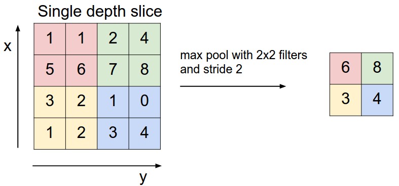
It is common to periodically insert a Pooling layer in-between successive Conv layers in a ConvNet architecture. The goal is: To progressively reduce the spatial size of the representation, thus to reduce the amount of parameters and computation, and hence to control overfitting. We use MAX operation to achieve these goals.
The most common form is a pooling layer with filters of size 2x2 applied with a stride of 2 downsamples every depth slice in the input by 2 along both width and height, discarding 75% of the activations. Every MAX operation would in this case be taking a max over 4 numbers (little 2x2 region in some depth slice). The depth dimension remains unchanged. More generally, the pooling layer:
Accepts a volume of size \( W_1 \times H_1 \times D_1 \).
Requires two hyperparameters:
1. their spatial extent \( F \),
2. the stride \( S \).
Introduces zero parameters since it computes a fixed function of the input.
For Pooling layers, it is not common to pad the input using zero-padding.
In most cases, \( F = 3 \), \( S = 2 \) (also called overlapping pooling), or more commonly \( F = 2 \), \( S = 2 \). Pooling sizes with larger receptive fields are too destructive.
defmax_pool_forward_naive(x,pool_param):"""A naive implementation of the forward pass for a max-pooling layer. Inputs: - x: Input data, of shape (N, C, H, W) - pool_param: dictionary with the following keys: - 'pool_height': The height of each pooling region - 'pool_width': The width of each pooling region - 'stride': The distance between adjacent pooling regions No padding is necessary here, eg you can assume: - (H - pool_height) % stride == 0 - (W - pool_width) % stride == 0 Returns a tuple of: - out: Output data, of shape (N, C, H', W') where H' and W' are given by H' = 1 + (H - pool_height) // stride W' = 1 + (W - pool_width) // stride - cache: (x, pool_param) """N,C,H,W=x.shapepool_height,pool_width,stride=pool_param['pool_height'],pool_param['pool_width'],pool_param['stride']H_out=1+(H-pool_height)//strideW_out=1+(W-pool_width)//strideout=np.zeros((N,C,H_out,W_out))forimage_indexinrange(N):forcinrange(C):foriinrange(H_out):forjinrange(W_out):i_start=i*stridej_start=j*stridei_end=i_start+pool_heightj_end=j_start+pool_width# Extract the region to poolregion=x[image_index,c,i_start:i_end,j_start:j_end]# Perform max poolingout[image_index,c,i,j]=np.max(region)cache=(x,pool_param)returnout,cachedefmax_pool_backward_naive(dout,cache):"""A naive implementation of the backward pass for a max-pooling layer. Inputs: - dout: Upstream derivatives of shape (N, C, H_out, W_out) - cache: A tuple of (x, pool_param) as in the forward pass. Returns: - dx: Gradient with respect to x, of shape (N, C, H, W) """x,pool_param=cacheN,C,H,W=x.shapepool_height,pool_width,stride=pool_param['pool_height'],pool_param['pool_width'],pool_param['stride']H_out=1+(H-pool_height)//strideW_out=1+(W-pool_width)//stridedx=np.zeros_like(x)forimage_indexinrange(N):forcinrange(C):foriinrange(H_out):forjinrange(W_out):i_start=i*stridej_start=j*stridei_end=i_start+pool_heightj_end=j_start+pool_width# Extract the region of the input that was pooledregion=x[image_index,c,i_start:i_end,j_start:j_end]# Find the mask of the maximum value in the regionmask=(region==np.max(region))# Distribute the gradient from dout to the corresponding max location in dxdx[image_index,c,i_start:i_end,j_start:j_end]+=mask*dout[image_index,c,i,j]returndx
Neurons in a fully connected layer have full connections to all activations in the previous layer, as seen in regular Neural Networks. Their activations can hence be computed with a matrix multiplication followed by a bias offset.
Important Note (Converting FC Layers to CONV Layers)
Note that the neurons in both FC layers and CONV layers compute dot products, so their functional form is identical. Therefore, it turns out that it’s possible to convert between FC and CONV layers. Of these two conversions, the ability to convert an FC layer to a CONV layer is particularly useful in practice. For example, an FC layer with \( K = 4096 \) that is looking at some input volume of size \( 7 \times 7 \times 512 \) can be equivalently expressed as a CONV layer with \( F = 7, P = 0, S = 1, K = 4096 \). In other words, we are setting the filter size to be exactly the size of the input volume, and hence the output will simply be \( 1 \times 1 \times 4096 \) since only a single depth column “fits” across the input volume, giving identical result as the initial FC layer.
Example (FC-CONV Conversion in AlexNet)
Consider a ConvNet architecture that takes a 224x224x3 image, and then uses a series of CONV layers and POOL layers to reduce the image to an activations volume of size 7x7x512 (in an AlexNet architecture that we’ll see later, this is done by use of 5 pooling layers that downsample the input spatially by a factor of two each time, making the final spatial size 224/2/2/2/2/2 = 7). From there, an AlexNet uses two FC layers of size 4096 and finally the last FC layers with 1000 neurons that compute the class scores. We can convert each of these three FC layers to CONV layers as described above:
Replace the first FC layer that looks at [7x7x512] volume with a CONV layer that uses filter size \( F = 7 \), giving output volume [1x1x4096].
Replace the second FC layer with a CONV layer that uses filter size \( F = 1 \), giving output volume [1x1x4096].
Replace the last FC layer similarly, with \( F = 1 \), giving final output [1x1x1000].
Each of these conversions could in practice involve manipulating (e.g. reshaping) the weight matrix \( W \) in each FC layer into CONV layer filters. It turns out that this conversion allows us to “slide” the original ConvNet very efficiently across many spatial positions in a larger image, in a single forward pass.
For example, if 224x224 image gives a volume of size [7x7x512] - i.e. a reduction by 32, then forwarding an image of size 384x384 through the converted architecture would give the equivalent volume in size [12x12x512], since 384/32 = 12. Following through with the next 3 CONV layers that we just converted from FC layers would now give the final volume of size [6x6x1000], since (12 - 7)/1 + 1 = 6. Note that instead of a single vector of class scores of size [1x1x1000], we’re now getting an entire 6x6 array of class scores across the 384x384 image.
Evaluating the original ConvNet (with FC layers) independently across 224x224 crops of the 384x384 image in strides of 32 pixels gives an identical result to forwarding the converted ConvNet one time.
Naturally, forwarding the converted ConvNet a single time is much more efficient than iterating the original ConvNet over all those 36 locations, since the 36 evaluations share computation. This trick is often used in practice to get better performance, where for example, it is common to resize an image to make it bigger, use a converted ConvNet to evaluate the class scores at many spatial positions and then average the class scores.
defaffine_forward(x,w,b):"""Computes the forward pass for an affine (fully connected) layer. The input x has shape (N, d_1, ..., d_k) and contains a minibatch of N examples, where each example x[i] has shape (d_1, ..., d_k). We will reshape each input into a vector of dimension D = d_1 * ... * d_k, and then transform it to an output vector of dimension M. Inputs: - x: A numpy array containing input data, of shape (N, d_1, ..., d_k) - w: A numpy array of weights, of shape (D, M) - b: A numpy array of biases, of shape (M,) Returns a tuple of: - out: output, of shape (N, M) - cache: (x, w, b) """out=Noneout=x.reshape(len(x),-1)@w+bcache=(x,w,b)returnout,cachedefaffine_backward(dout,cache):"""Computes the backward pass for an affine (fully connected) layer. Inputs: - dout: Upstream derivative, of shape (N, M) - cache: Tuple of: - x: Input data, of shape (N, d_1, ... d_k) - w: Weights, of shape (D, M) - b: Biases, of shape (M,) Returns a tuple of: - dx: Gradient with respect to x, of shape (N, d1, ..., d_k) - dw: Gradient with respect to w, of shape (D, M) - db: Gradient with respect to b, of shape (M,) """x,w,b=cachedx,dw,db=None,None,Nonedx=(dout@w.T).reshape(x.shape)dw=x.reshape(len(x),-1).T@doutdb=dout.sum(axis=0)returndx,dw,db
defsoftmax_loss(x,y):"""Computes the loss and gradient for softmax classification.Inputs:-x:Inputdata,ofshape(N,C)wherex[i,j]isthescoreforthejthclassfortheithinput.-y:Vectoroflabels,ofshape(N,)wherey[i]isthelabelforx[i]and0<=y[i]<CReturnsatupleof:-loss:Scalargivingtheloss-dx:Gradientofthelosswithrespecttox"""loss,dx=None,NoneN=len(y)#numberofsamplesP=np.exp(x-x.max(axis=1,keepdims=True))#numericallystableexponentsP/=P.sum(axis=1,keepdims=True)#row-wiseprobabilities(softmax)loss=-np.log(P[range(N),y]).sum()/N#sumcrossentropiesaslossP[range(N),y]-=1dx=P/Nreturnloss,dx
defbatchnorm_forward(x,gamma,beta,bn_param):"""Forward pass for batch normalization. During training the sample mean and (uncorrected) sample variance are computed from minibatch statistics and used to normalize the incoming data. During training we also keep an exponentially decaying running mean of the mean and variance of each feature, and these averages are used to normalize data at test-time. At each timestep we update the running averages for mean and variance using an exponential decay based on the momentum parameter: running_mean = momentum * running_mean + (1 - momentum) * sample_mean running_var = momentum * running_var + (1 - momentum) * sample_var Note that the batch normalization paper suggests a different test-time behavior: they compute sample mean and variance for each feature using a large number of training images rather than using a running average. For this implementation we have chosen to use running averages instead since they do not require an additional estimation step; the torch7 implementation of batch normalization also uses running averages. Input: - x: Data of shape (N, D) - gamma: Scale parameter of shape (D,) - beta: Shift paremeter of shape (D,) - bn_param: Dictionary with the following keys: - mode: 'train' or 'test'; required - eps: Constant for numeric stability - momentum: Constant for running mean / variance. - running_mean: Array of shape (D,) giving running mean of features - running_var Array of shape (D,) giving running variance of features Returns a tuple of: - out: of shape (N, D) - cache: A tuple of values needed in the backward pass """mode=bn_param["mode"]eps=bn_param.get("eps",1e-5)momentum=bn_param.get("momentum",0.9)N,D=x.shaperunning_mean=bn_param.get("running_mean",np.zeros(D,dtype=x.dtype))running_var=bn_param.get("running_var",np.zeros(D,dtype=x.dtype))out,cache=None,Noneifmode=="train":mu=x.mean(axis=0)var=x.var(axis=0)std=np.sqrt(var+eps)x_new=(x-mu)/stdout=gamma*x_new+betashape=bn_param.get('shape',(N,D))# reshape used in backpropaxis=bn_param.get('axis',0)# axis to sum used in backpropcache=x,mu,var,std,gamma,x_new,shape,axis# save for backpropifaxis==0:# if not batchnormrunning_mean=momentum*running_mean+(1-momentum)*mu# update overall meanrunning_var=momentum*running_var+(1-momentum)*var# update overall varianceelifmode=="test":x_new=(x-running_mean)/np.sqrt(running_var+eps)out=gamma*x_new+betaelse:raiseValueError('Invalid forward batchnorm mode "%s"'%mode)# Store the updated running means back into bn_parambn_param["running_mean"]=running_meanbn_param["running_var"]=running_varreturnout,cachedefbatchnorm_backward(dout,cache):"""Backward pass for batch normalization. For this implementation, you should write out a computation graph for batch normalization on paper and propagate gradients backward through intermediate nodes. Inputs: - dout: Upstream derivatives, of shape (N, D) - cache: Variable of intermediates from batchnorm_forward. Returns a tuple of: - dx: Gradient with respect to inputs x, of shape (N, D) - dgamma: Gradient with respect to scale parameter gamma, of shape (D,) - dbeta: Gradient with respect to shift parameter beta, of shape (D,) """dx,dgamma,dbeta=None,None,Nonex,mu,var,std,gamma,x_hat,shape,axis=cache# expand cachedbeta=dout.reshape(shape,order='F').sum(axis)# derivative w.r.t. betadgamma=(dout*x_hat).reshape(shape,order='F').sum(axis)# derivative w.r.t. gammadx_hat=dout*gamma# derivative w.t.r. x_hatdstd=-np.sum(dx_hat*(x-mu),axis=0)/(std**2)# derivative w.t.r. stddvar=0.5*dstd/std# derivative w.t.r. vardx1=dx_hat/std+2*(x-mu)*dvar/len(dout)# partial derivative w.t.r. dxdmu=-np.sum(dx1,axis=0)# derivative w.t.r. mudx2=dmu/len(dout)# partial derivative w.t.r. dxdx=dx1+dx2# full derivative w.t.r. xreturndx,dgamma,dbetadefbatchnorm_backward_alt(dout,cache):"""Alternative backward pass for batch normalization. For this implementation you should work out the derivatives for the batch normalizaton backward pass on paper and simplify as much as possible. You should be able to derive a simple expression for the backward pass. See the jupyter notebook for more hints. Note: This implementation should expect to receive the same cache variable as batchnorm_backward, but might not use all of the values in the cache. Inputs / outputs: Same as batchnorm_backward """dx,dgamma,dbeta=None,None,None_,_,_,std,gamma,x_hat,shape,axis=cache# expand cacheS=lambdax:x.sum(axis=0)# helper functiondbeta=dout.reshape(shape,order='F').sum(axis)# derivative w.r.t. betadgamma=(dout*x_hat).reshape(shape,order='F').sum(axis)# derivative w.r.t. gammadx=dout*gamma/(len(dout)*std)# temporarily initialize scale valuedx=len(dout)*dx-S(dx*x_hat)*x_hat-S(dx)# derivative w.r.t. unnormalized xreturndx,dgamma,dbeta
deflayernorm_forward(x,gamma,beta,ln_param):"""Forward pass for layer normalization. During both training and test-time, the incoming data is normalized per data-point, before being scaled by gamma and beta parameters identical to that of batch normalization. Note that in contrast to batch normalization, the behavior during train and test-time for layer normalization are identical, and we do not need to keep track of running averages of any sort. Input: - x: Data of shape (N, D) - gamma: Scale parameter of shape (D,) - beta: Shift paremeter of shape (D,) - ln_param: Dictionary with the following keys: - eps: Constant for numeric stability Returns a tuple of: - out: of shape (N, D) - cache: A tuple of values needed in the backward pass """out,cache=None,Noneeps=ln_param.get("eps",1e-5)bn_param={"mode":"train","axis":1,**ln_param}# same as batchnorm in train mode + over which axis to sum for grad[gamma,beta]=np.atleast_2d(gamma,beta)# assure 2D to perform transposeout,cache=batchnorm_forward(x.T,gamma.T,beta.T,bn_param)# same as batchnormout=out.T# transpose backreturnout,cachedeflayernorm_backward(dout,cache):"""Backward pass for layer normalization. For this implementation, you can heavily rely on the work you've done already for batch normalization. Inputs: - dout: Upstream derivatives, of shape (N, D) - cache: Variable of intermediates from layernorm_forward. Returns a tuple of: - dx: Gradient with respect to inputs x, of shape (N, D) - dgamma: Gradient with respect to scale parameter gamma, of shape (D,) - dbeta: Gradient with respect to shift parameter beta, of shape (D,) """dx,dgamma,dbeta=None,None,Nonedx,dgamma,dbeta=batchnorm_backward_alt(dout.T,cache)# same as batchnorm backpropdx=dx.Treturndx,dgamma,dbeta