Nearest Neighbor Classifier is very rarely used in practice, but it will allow us to get an idea about the basic approach to an image classification problem.
Important Note (CIFAR-10 Dataset)
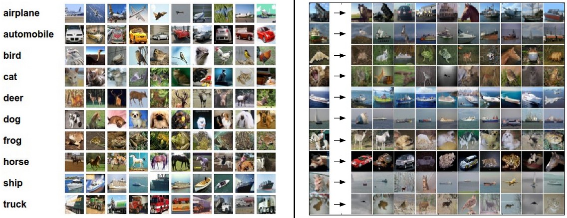
One popular toy image classification dataset is the CIFAR-10 dataset. This dataset consists of 60,000 tiny images that are 32 pixels high and wide. Each image is labeled with one of 10 classes (for example “airplane, automobile, bird, etc”). These 60,000 images are partitioned into a training set of 50,000 images and a test set of 10,000 images.
importrandomimportnumpyasnpfromcs231n.data_utilsimportload_CIFAR10importmatplotlib.pyplotasplt# This is a bit of magic to make matplotlib figures appear inline in the notebook# rather than in a new window.%matplotlibinlineplt.rcParams['figure.figsize']=(10.0,8.0)# set default size of plotsplt.rcParams['image.interpolation']='nearest'plt.rcParams['image.cmap']='gray'# Some more magic so that the notebook will reload external python modules;# see http://stackoverflow.com/questions/1907993/autoreload-of-modules-in-ipython%load_extautoreload%autoreload2# Load the raw CIFAR-10 data.cifar10_dir='cs231n/datasets/cifar-10-batches-py'# Cleaning up variables to prevent loading data multiple times (which may cause memory issue)try:delX_train,y_traindelX_test,y_testprint('Clear previously loaded data.')except:passX_train,y_train,X_test,y_test=load_CIFAR10(cifar10_dir)# As a sanity check, we print out the size of the training and test data.print('Training data shape: ',X_train.shape)print('Training labels shape: ',y_train.shape)print('Test data shape: ',X_test.shape)print('Test labels shape: ',y_test.shape)
Important Note (Visualizing CIFAR-10)
1 2 3 4 5 6 7 8 910111213141516
# Visualize some examples from the dataset.# We show a few examples of training images from each class.classes=['plane','car','bird','cat','deer','dog','frog','horse','ship','truck']num_classes=len(classes)samples_per_class=7fory,clsinenumerate(classes):idxs=np.flatnonzero(y_train==y)idxs=np.random.choice(idxs,samples_per_class,replace=False)fori,idxinenumerate(idxs):plt_idx=i*num_classes+y+1plt.subplot(samples_per_class,num_classes,plt_idx)plt.imshow(X_train[idx].astype('uint8'))plt.axis('off')ifi==0:plt.title(cls)plt.show()
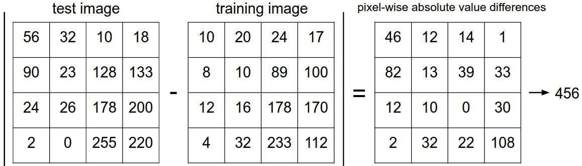
Before introducing algorithms to solve an image classification problem, we need to first define the difference between two images. One of the simplest possibilities is to compare the images pixel by pixel and add up all the differences.
Definition (L1 Distance)
Given two images and representing them as vectors \(I_1, I_2\), a reasonable choice for comparing them might be the L1 distance:
\[d_1(I_1, I_2) = \sum_p |I_1^p - I_2^p|\]
Here is the procedure visualized:
There are many other ways of computing distances between vectors. Another common choice could be to instead use the L2 distance, which has the geometric interpretation of computing the Euclidean distance between two vectors.
Suppose now that we are given the CIFAR-10 training set of 50,000 images (5,000 images for every one of the labels), and we wish to label the remaining 10,000. The nearest neighbor classifier will take a test image, compare it to every single one of the training images, and predict the label of the closest training image. In the image "CIFAR-10 Dataset" you can see an example result of such a procedure for 10 example test images.
Note (Performance of Nearest Neighbor Classifier)
If you ran the Nearest Neighbor classifier on CIFAR-10 with L2 distance, you would obtain 35.4% accuracy (slightly lower than our L1 distance result - 38.6%).
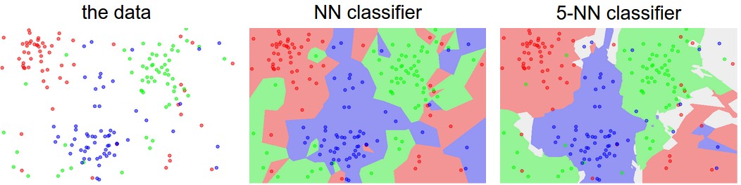
You may have noticed that it is strange to only use the label of the nearest image when we wish to make a prediction. Indeed, it is almost always the case that one can do better by using what’s called a k-Nearest Neighbor Classifier.
Definition (k - Nearest Neighbor Classifier)
instead of finding the single closest image in the training set, we will find the top k closest images, and have them vote on the label of the test image. In particular, when k = 1, we recover the Nearest Neighbor classifier. Intuitively, higher values of k have a smoothing effect that makes the classifier more resistant to outliers:
k - Nearest Neighbor Classifier
Important Note (Implementing kNN)
In train method, we train the model, i.e. get the trained parameters. However, in kNN, we are just memorizing the training data:
1 2 3 4 5 6 7 8 910
deftrain(self,X,y):""" Inputs: - X: A numpy array of shape (num_train, D) containing the training data consisting of num_train samples each of dimension D. - y: A numpy array of shape (N,) containing the training labels, where y[i] is the label for X[i]. """self.X_train=Xself.y_train=y
Next is our predict method, which is to predict labels for test data. Note that as the first classifier to implement, we all use three different methods to calculate distances:
1 2 3 4 5 6 7 8 91011121314151617181920212223
defpredict(self,X,k=1,num_loops=0):""" Inputs: - X: A numpy array of shape (num_test, D) containing test data consisting of num_test samples each of dimension D. - k: The number of nearest neighbors that vote for the predicted labels. - num_loops: Determines which implementation to use to compute distances between training points and testing points. Returns: - y: A numpy array of shape (num_test,) containing predicted labels for the test data, where y[i] is the predicted label for the test point X[i]. """ifnum_loops==0:dists=self.compute_distances_no_loops(X)elifnum_loops==1:dists=self.compute_distances_one_loop(X)elifnum_loops==2:dists=self.compute_distances_two_loops(X)else:raiseValueError("Invalid value %d for num_loops"%num_loops)returnself.predict_labels(dists,k=k)
We now use a naive way of computing dists with two loops (very slow):
1 2 3 4 5 6 7 8 9101112131415161718192021222324
defcompute_distances_two_loops(self,X):""" Compute the distance between each test point in X and each training point in self.X_train using a nested loop over both the training data and the test data. Inputs: - X: A numpy array of shape (num_test, D) containing test data. Returns: - dists: A numpy array of shape (num_test, num_train) where dists[i, j] is the Euclidean distance between the ith test point and the jth training point. """num_test=X.shape[0]num_train=self.X_train.shape[0]dists=np.zeros((num_test,num_train))foriinrange(num_test):forjinrange(num_train):# Compute the l2 distance between the ith test point and the jth# training point, and store the result in dists[i, j]. dists[i,j]=np.sqrt(np.sum(np.square(X[i]-self.X_train[j])))returndists
Now we try to use only one loop (not necessarily faster than two loops, however):
defpredict_labels(self,dists,k=1):""" Given a matrix of distances between test points and training points, predict a label for each test point. Inputs: - dists: A numpy array of shape (num_test, num_train) where dists[i, j] gives the distance betwen the ith test point and the jth training point. Returns: - y: A numpy array of shape (num_test,) containing predicted labels for the test data, where y[i] is the predicted label for the test point X[i]. """num_test=dists.shape[0]y_pred=np.zeros(num_test)foriinrange(num_test):# A list of length k storing the labels of the k nearest neighbors to# the ith test point.closest_y=[]# Use the distance matrix to find the k nearest neighbors of the ith ## testing point, and use self.y_train to find the labels of these ## neighbors. Store these labels in closest_y. closest_y=self.y_train[np.argsort(dists[i])[:k]]# Now that you have found the labels of the k nearest neighbors, you ## need to find the most common label in the list closest_y of labels. ## Store this label in y_pred[i]. Break ties by choosing the smaller ## label. #y_pred[i]=np.argmax(np.bincount(closest_y))returny_pred
frombuiltinsimportrangefrombuiltinsimportobjectimportnumpyasnpfrompast.builtinsimportxrangeclassKNearestNeighbor(object):""" a kNN classifier with L2 distance """def__init__(self):passdeftrain(self,X,y):""" Train the classifier. For k-nearest neighbors this is just memorizing the training data. Inputs: - X: A numpy array of shape (num_train, D) containing the training data consisting of num_train samples each of dimension D. - y: A numpy array of shape (N,) containing the training labels, where y[i] is the label for X[i]. """self.X_train=Xself.y_train=ydefpredict(self,X,k=1,num_loops=0):""" Predict labels for test data using this classifier. Inputs: - X: A numpy array of shape (num_test, D) containing test data consisting of num_test samples each of dimension D. - k: The number of nearest neighbors that vote for the predicted labels. - num_loops: Determines which implementation to use to compute distances between training points and testing points. Returns: - y: A numpy array of shape (num_test,) containing predicted labels for the test data, where y[i] is the predicted label for the test point X[i]. """ifnum_loops==0:dists=self.compute_distances_no_loops(X)elifnum_loops==1:dists=self.compute_distances_one_loop(X)elifnum_loops==2:dists=self.compute_distances_two_loops(X)else:raiseValueError("Invalid value %d for num_loops"%num_loops)returnself.predict_labels(dists,k=k)defcompute_distances_two_loops(self,X):""" Compute the distance between each test point in X and each training point in self.X_train using a nested loop over both the training data and the test data. Inputs: - X: A numpy array of shape (num_test, D) containing test data. Returns: - dists: A numpy array of shape (num_test, num_train) where dists[i, j] is the Euclidean distance between the ith test point and the jth training point. """num_test=X.shape[0]num_train=self.X_train.shape[0]dists=np.zeros((num_test,num_train))foriinrange(num_test):forjinrange(num_train):# Compute the l2 distance between the ith test point and the jth ## training point, and store the result in dists[i, j]. You should ## not use a loop over dimension, nor use np.linalg.norm(). #dists[i,j]=np.sqrt(np.sum(np.square(X[i]-self.X_train[j])))returndistsdefcompute_distances_one_loop(self,X):""" Compute the distance between each test point in X and each training point in self.X_train using a single loop over the test data. Input / Output: Same as compute_distances_two_loops """num_test=X.shape[0]num_train=self.X_train.shape[0]dists=np.zeros((num_test,num_train))foriinrange(num_test):# Compute the l2 distance between the ith test point and all training ## points, and store the result in dists[i, :]. #dists[i]=np.sqrt(np.sum(np.square(X[i]-self.X_train),axis=1))returndistsdefcompute_distances_no_loops(self,X):""" Compute the distance between each test point in X and each training point in self.X_train using no explicit loops. Input / Output: Same as compute_distances_two_loops """num_test=X.shape[0]num_train=self.X_train.shape[0]dists=np.zeros((num_test,num_train))# Compute the l2 distance between all test points and all training ## points without using any explicit loops, and store the result in ## dists. #dists=np.sqrt(-2*(X@self.X_train.T)+np.square(X).sum(axis=1,keepdims=True)+np.square(self.X_train).sum(axis=1,keepdims=True).T)returndistsdefpredict_labels(self,dists,k=1):""" Given a matrix of distances between test points and training points, predict a label for each test point. Inputs: - dists: A numpy array of shape (num_test, num_train) where dists[i, j] gives the distance betwen the ith test point and the jth training point. Returns: - y: A numpy array of shape (num_test,) containing predicted labels for the test data, where y[i] is the predicted label for the test point X[i]. """num_test=dists.shape[0]y_pred=np.zeros(num_test)foriinrange(num_test):# A list of length k storing the labels of the k nearest neighbors to# the ith test point.closest_y=[]# Use the distance matrix to find the k nearest neighbors of the ith ## testing point, and use self.y_train to find the labels of these ## neighbors. Store these labels in closest_y. ## Hint: Look up the function numpy.argsort. #closest_y=self.y_train[np.argsort(dists[i])[:k]]y_pred[i]=np.argmax(np.bincount(closest_y))returny_pred
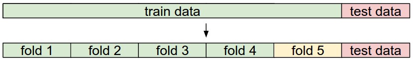
Definition (Validation Set)
There is a correct way of tuning the hyperparameters and it does not touch the test set at all. The idea is to split our training set in two: a slightly smaller training set, and what we call a validation set. Using CIFAR-10 as an example, we could for example use 49,000 of the training images for training, and leave 1,000 aside for validation. This validation set is essentially used as a fake test set to tune the hyper-parameters.
Split your training set into training set and a validation set. Use validation set to tune all hyperparameters. At the end run a single time on the test set and report performance.
Definition (Cross-Validation)
In cases where the size of your training data (and therefore also the validation data) might be small, people sometimes use a more sophisticated technique for hyperparameter tuning called cross-validation. Working with our previous example, the idea is that instead of arbitrarily picking the first 1000 datapoints to be the validation set and rest training set, you can get a better and less noisy estimate of how well a certain value of k works by iterating over different validation sets and averaging the performance across these. For example, in 5-fold cross-validation, we would split the training data into 5 equal folds, use 4 of them for training, and 1 for validation. We would then iterate over which fold is the validation fold, evaluate the performance, and finally average the performance across the different folds.
Important Note (Implementing Cross-Validation to Find The Best k Value)
num_folds=5k_choices=[1,3,5,8,10,12,15,20,50,100]X_train_folds=[]y_train_folds=[]X_train_folds=np.array_split(X_train,num_folds)y_train_folds=np.array_split(y_train,num_folds)# A dictionary holding the accuracies for different values of k that we find# when running cross-validation. After running cross-validation,# k_to_accuracies[k] should be a list of length num_folds giving the different# accuracy values that we found when using that value of k.k_to_accuracies={}# Perform k-fold cross validation to find the best value of k. For each ## possible value of k, run the k-nearest-neighbor algorithm num_folds times, ## where in each case you use all but one of the folds as training data and the ## last fold as a validation set. Store the accuracies for all fold and all ## values of k in the k_to_accuracies dictionary. #forkink_choices:k_to_accuracies[k]=[]foriinrange(num_folds):X_train_temp=np.concatenate(np.compress(np.arange(num_folds)!=i,X_train_folds,axis=0))y_train_temp=np.concatenate(np.compress(np.arange(num_folds)!=i,y_train_folds,axis=0))classifier.train(X_train_temp,y_train_temp)y_pred_temp=classifier.predict(X_train_folds[i],k=k)num_correct=np.sum(y_pred_temp==y_train_folds[i])accuracy=float(num_correct)/len(y_train_folds[i])k_to_accuracies[k].append(accuracy)# Print out the computed accuraciesforkinsorted(k_to_accuracies):foraccuracyink_to_accuracies[k]:print('k = %d, accuracy = %f'%(k,accuracy))
Important Note (In Practice)
In practice, people prefer to avoid cross-validation in favor of having a single validation split, since cross-validation can be computationally expensive. The splits people tend to use is between 50%-90% of the training data for training and rest for validation. However, this depends on multiple factors: For example if the number of hyperparameters is large you may prefer to use bigger validation splits. If the number of examples in the validation set is small (perhaps only a few hundred or so), it is safer to use cross-validation. Typical number of folds you can see in practice would be 3-fold, 5-fold or 10-fold cross-validation.
Common Data Splits
Note (Final Accuracy of kNN)
After using cross-validation, we found that the best k value is 10, which leads to the final accuracy of kNN: 0.282.
Important Note (Pros and Cons of NN)
The nearest neighbor classifier takes no time to train, since all that is required is to store and possibly index the training data. However, we pay that computational cost at test time, since classifying a test example requires a comparison to every single training example.
Important Note (Problems of NN)
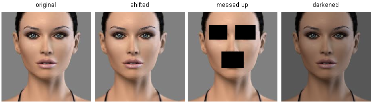
Images are high-dimensional objects (i.e. they often contain many pixels), and distances over high-dimensional spaces can be very counter-intuitive. The image below illustrates the point that the pixel-based L2 similarities we developed above are very different from perceptual similarities:
Here is one more visualization to convince you that using pixel differences to compare images is inadequate. We can use a visualization technique called t-SNE to take the CIFAR-10 images and embed them in two dimensions so that their (local) pairwise distances are best preserved. In this visualization, images that are shown nearby are considered to be very near according to the L2 pixelwise distance we developed above:
In particular, note that images that are nearby each other are much more a function of the general color distribution of the images, or the type of background rather than their semantic identity.