Linear Classifiers
Interpreting Linear Classifiers
Important Note (Naive Interpretation of Linear Classifiers)
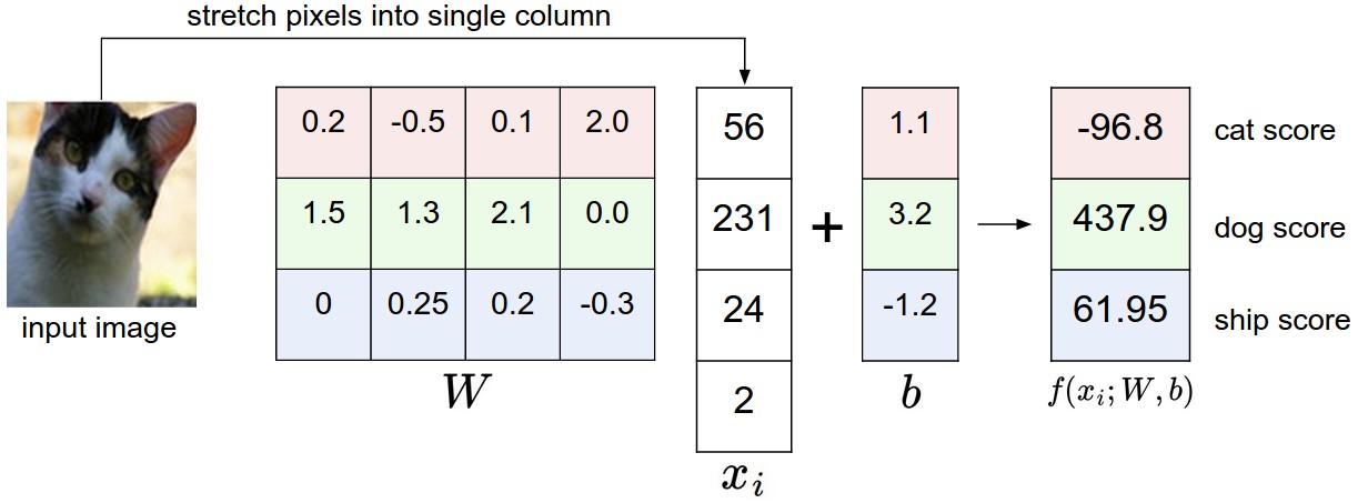
A linear classifier computes the score of a class as a weighted sum of all of its pixel values across all 3 of its color channels. The function has the capacity to like or dislike (the sign of each weight) certain colors at certain positions in the image. For instance, the “ship” class might be more likely if there is a lot of blue on the sides of an image. The “ship” classifier would then have a lot of positive weights across its blue channel weights, and negative weights in the red/green channels.
Important Note (Analogy of Images as High-Dimensional Points.)
Since the images are stretched into high-dimensional column vectors, we can interpret each image as a single point in this space (e.g. each image in CIFAR-10 is a point in 3072-dimensional space of 32x32x3 pixels).
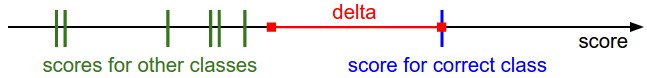
Since we defined the score of each class as a weighted sum of all image pixels, each class score is a linear function over this space. We cannot visualize 3072-dimensional spaces, but if we imagine squashing all those dimensions into only two dimensions, then we can try to visualize what the classifier might be doing:
![]()
Using the example of the car classifier (in red), the red line shows all points in the space that get a score of zero for the car class. The red arrow shows the direction of increase, so all points to the right of the red line have positive (and linearly increasing) scores, and all points to the left have a negative (and linearly decreasing) scores.
Important Note (Interpretation of Linear Classifiers as Template Matching)
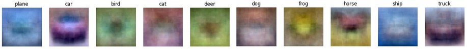
Another interpretation for the weights \(\mathbf{W}\) is that each row of \(\mathbf{W}\) corresponds to a template for one of the classes. The score of each class for an image is then obtained by comparing each template with the image using dot product one by one to find the one that “fits” best. With this terminology, the linear classifier is doing template matching, where the templates are learned.
Another way to think of it is that we are still effectively doing Nearest Neighbor, but instead of having thousands of training images we are only using a single image per class (although we will learn it, and it does not necessarily have to be one of the images in the training set), and we use the (negative) inner product as the distance instead of the L1 or L2 distance.
Note (Observation in Templates)
Note that the horse template seems to contain a two-headed horse, which is due to both left and right facing horses in the dataset. The linear classifier merges these two modes of horses in the data into a single template. Similarly, the car classifier seems to have merged several modes into a single template which has to identify cars from all sides, and of all colors. In particular, this template ended up being red, which hints that there are more red cars in the CIFAR-10 dataset than of any other color. The linear classifier is too weak to properly account for different-colored cars, but neural networks will allow us to perform this task.
Strategy (Bias Trick)
Recall that we defined the score function as:
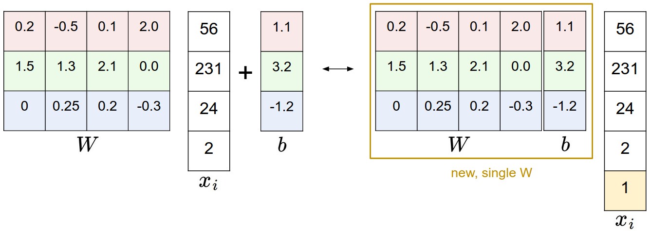
A commonly used trick is to combine the two sets of parameters into a single matrix that holds both of them by extending the vector \(x_i\) with one additional dimension that always holds the constant 1 - a default bias dimension. With the extra dimension, the new score function will simplify to a single matrix multiply:
With our CIFAR-10 example, \(x_i\) is now [3073 x 1] instead of [3072 x 1] - (with the extra dimension holding the constant 1), and \(W\) is now [10 x 3073] instead of [10 x 3072]. The extra column that \(W\) now corresponds to the bias \(b\). An illustration might help clarify:
Strategy (Normalization of Input Features)
In Machine Learning, it is a very common practice to always perform normalization of input features (in the case of images, every pixel is thought of as a feature). In particular, it is important to center your data by subtracting the mean from every feature. In the case of images, this corresponds to computing a mean image across the training images and subtracting it from every image to get images where the pixels range from approximately [-127 … 127]. Further common preprocessing is to scale each input feature so that its values range from [-1, 1]. Of these, zero mean centering is arguably more important but we will talk about it later.
Multiclass Support Vector Machine (SVM) Loss
The SVM loss is set up so that the SVM “wants” the correct class for each image to have a score higher than the incorrect classes by some fixed margin \(\Delta\).
Definition (SVM Loss)
Recall that for the i-th example we are given the pixels of image \(x_i\) and the label \(y_i\) that specifies the index of the correct class. The score function takes the pixels and computes the vector \(f(x_i, W)\) of class scores, which we will abbreviate to \(\mathbf{s}\) (short for scores). For example, the score for the j-th class is the j-th element: \(s_j = f(x_i, W)_j\). The Multiclass SVM loss for the i-th example is then formalized as follows:
Note that in this particular module we are working with linear score functions \(( f(x_i; W) = W x_i )\), so we can also rewrite the loss function in this equivalent form:
where \(\mathbf{w}_j\) is the j-th row of \(W\) reshaped as a column. However, this will not necessarily be the case once we start to consider more complex forms of the score function \(f\).
Example (Example of SVM Loss)
Suppose that we have three classes that receive the scores \(\mathbf{s} = [13, -7, 11]\), and that the first class is the true class (i.e. \(y_i = 0\)). Also assume that \(\Delta\) (a hyperparameter we will go into more detail about soon) is 10. The expression above sums over all incorrect classes \((j \ne y_i)\), so we get two terms:
You can see that the first term gives zero since \([-7 - 13 + 10]\) gives a negative number, which is then thresholded to zero with the \(\max(0, -)\) function. We get zero loss for this pair because the correct class score (13) was greater than the incorrect class score (-7) by at least the margin 10. In fact the difference was 20, which is much greater than 10 but the SVM only cares that the difference is at least 10; Any additional difference above the margin is clamped at zero with the max operation. The second term computes \([11 - 13 + 10]\) which gives 8. That is, even though the correct class had a higher score than the incorrect class \((13 > 11)\), it was not greater by the desired margin of 10. The difference was only 2, which is why the loss comes out to 8 (i.e. how much higher the difference would have to be to meet the margin). In summary, the SVM loss function wants the score of the correct class \(y_i\) to be larger than the incorrect class scores by at least \(\Delta\) (delta). If this is not the case, we will accumulate loss.
Definition (Hinge Loss)
When the threshold is at zero, i.e. \(\max(0, -)\), the function is often called the Hinge Loss. You’ll sometimes hear about people instead using the squared hinge loss SVM (or L2-SVM), which uses the form \(\max(0, -)^2\) that penalizes violated margins more strongly (quadratically instead of linearly). The unsquared version is more standard, but in some datasets the squared hinge loss can work better. This can be determined during cross-validation.
Regularization
There is one bug with the loss function we presented above. Suppose that we have a dataset and a set of parameters \(W\) that correctly classify every example (i.e. all scores are so that all the margins are met, and \(L_i = 0\) for all \(i\)). The issue is that this set of \(W\) is not necessarily unique: there might be many similar \(W\) that correctly classify the examples. For example, \(2W\).
In other words, we wish to encode some preference for a certain set of weights \(W\) over others to remove this ambiguity. We can do so by extending the loss function with a regularization penalty \(R(W)\).
The most common regularization penalty is the squared L2 norm.
Definition (L2 Regularization)
L2 Regularization discourages large weights through an elementwise quadratic penalty over all parameters:
Including the regularization penalty completes the full Multiclass Support Vector Machine loss, which is made up of two components: the data loss (which is the average loss \(L_i\) over all examples) and the regularization loss. That is, the full Multiclass SVM loss becomes:
Or expanding this out in its full form:
Where \(N\) is the number of training examples. As you can see, we append the regularization penalty to the loss objective, weighted by a hyperparameter \(\lambda\). There is no simple way of setting this hyperparameter and it is usually determined by cross-validation.
In addition to the motivation we provided above there are many desirable properties to include the regularization penalty, many of which we will come back to in later sections. For example, it turns out that including the L2 penalty leads to the appealing max margin property in SVMs.
Important Note (Why Regularization?)
The most appealing property is that penalizing large weights tends to improve generalization, because it means that no input dimension can have a very large influence on the scores all by itself.
Example (Why Not Regularization?)
Suppose that we have some input vector \(\mathbf{x} = [1, 1, 1, 1]\) and two weight vectors \(\mathbf{w}_1 = [1, 0, 0, 0]\), \(\mathbf{w}_2 = [0.25, 0.25, 0.25, 0.25]\). Then \(\mathbf{w}_1^T \mathbf{x} = \mathbf{w}_2^T \mathbf{x} = 1\) so both weight vectors lead to the same dot product, but the L2 penalty of \(\mathbf{w}_1\) is 1.0 while the L2 penalty of \(\mathbf{w}_2\) is only 0.5. Therefore, according to the L2 penalty the weight vector \(\mathbf{w}_2\) would be preferred since it achieves a lower regularization loss. Intuitively, this is because the weights in \(\mathbf{w}_2\) are smaller and more diffuse. Since the L2 penalty prefers smaller and more diffuse weight vectors, the final classifier is encouraged to take into account all input dimensions to small amounts rather than a few input dimensions very strongly.
wait, if we prefer more difused weights, doesn't the model overfit more since we include more features and count for subtle difference?
Note (Biases v.s. Penalty)
Note that biases do not have the same effect as penalty, since, unlike the weights, they do not control the strength of influence of an input dimension. Therefore, it is common to only regularize the weights \(W\) but not the biases \(b\). However, in practice this often turns out to have a negligible effect.
Note (0 Loss Impossible with Regularization)
Note that due to the regularization penalty we can never achieve loss of exactly 0.0 on all examples, because this would only be possible in the pathological setting of \(W = 0\).