Logistic Regression

Recall that we have discussed the sigmoid function, which is also known as the logistic function. We will discuss how to build up a regression based on that for a classification problem.

Logistic Regression

Model (Logistic Regression)

Consider a classification problem where \(y \in \{0,1\}\). Define

\[\begin{align*} g(z) = \frac{1}{1+e^{-z}} \end{align*}\]

We change our hypotheses \(h_{\theta}(x)\) to

\[\begin{align*} h_{\theta}(x) = g(\theta^Tx) = \frac{1}{1 + e^{-\theta^Tx}} \end{align*}\]

We pretend \(h_{\theta}(x)\) to be the probability of \(y = 1\).
Recall that

\[\begin{align*} g'(z) &= \frac{d}{dz}\frac{1}{1+e^{-z}} \\ &= \frac{1}{(1+e^{-z})^2}(e^{-z}) \\ &= \frac{1}{1+e^{-z}}\cdot (1-\frac{1}{1+e^{-z}}) \\ &= g(z)(1-g(z)) \end{align*}\]

Similar to MLE in linear regression, let us assume

\[\begin{align*} P(y=1\mid x;\theta) &= h_{\theta}(x) \\ P(y=0\mid x;\theta) &= 1 - h_{\theta}(x) \end{align*}\]

which is equivalent to

\[\begin{align*} p(y \mid x;\theta) = (h_{\theta}(x))^y(1-h_{\theta}(x))^{1-y} \end{align*}\]

By IID assumption, the likelihood of the parameters is:

\[\begin{align*} L(\theta) &= p(\hat{y}\mid X;\theta) \\ &= \prod_{i=1}^{n} p(y^{(i)} | x^{(i)}; \theta) \\ &= \prod_{i=1}^{n} (h_{\theta}(x^{(i)}))^{y^{(i)}} (1 - h_{\theta}(x^{(i)}))^{1 - y^{(i)}} \\ \end{align*}\]

Transform this into log likelihood:

\[\begin{align*} \ell(\theta) &= \log L(\theta) \\ &= \log \left( \prod_{i=1}^{n} (h_{\theta}(x^{(i)}))^{y^{(i)}} (1 - h_{\theta}(x^{(i)}))^{1 - y^{(i)}} \right) \\ &= \sum_{i=1}^{n} \log \left( (h_{\theta}(x^{(i)}))^{y^{(i)}} (1 - h_{\theta}(x^{(i)}))^{1 - y^{(i)}} \right) \\ &= \sum_{i=1}^{n} \left( y^{(i)} \log h_{\theta}(x^{(i)}) + (1 - y^{(i)}) \log (1 - h_{\theta}(x^{(i)})) \right) \\ &= \sum_{i=1}^{n} \left( y^{(i)} \log h_{\theta}(x^{(i)}) + (1 - y^{(i)}) \log (1 - h_{\theta}(x^{(i)})) \right) \end{align*}\]

To maximize the likelihood, we use gradient ascent. The equation to update \(\theta\) is:

\[\begin{align*} \theta := \theta + \alpha \nabla_{\theta} \ell(\theta) \end{align*}\]

Now, let us calculate the partial derivative of \(\ell(\theta)\) with repect to \(\theta_j\). Remember that \(g'(z) = g(z)(1-g(z))\):

\[\begin{align*} \frac{\partial}{\partial \theta_j} \ell(\theta) &= \left( \frac{y}{g(\theta^T x)} - \frac{(1 - y)}{1 - g(\theta^T x)} \right) \frac{\partial}{\partial \theta_j} g(\theta^T x) \\ &= \left( \frac{y}{g(\theta^T x)} - \frac{(1 - y)}{1 - g(\theta^T x)} \right) g(\theta^T x) (1 - g(\theta^T x)) \frac{\partial}{\partial \theta_j} \theta^T x \\ &= \left( \frac{y}{g(\theta^T x)} - \frac{(1 - y)}{1 - g(\theta^T x)} \right) g(\theta^T x) (1 - g(\theta^T x)) x_j \\ &= \left( y (1 - g(\theta^T x)) - (1 - y) g(\theta^T x) \right) x_j \\ &= (y - h_{\theta}(x)) x_j \end{align*}\]

Using the above partial derivative, we update \(\theta_j\) using the stochastic gradient ascent rule:

\[ \theta_j := \theta_j + \alpha \left( y^{(i)} - h_{\theta}(x^{(i)}) \right) x_j^{(i)} \]

Important Note (Comparing Logistic and Linear Regression)

Method	Distribution	Problem Type	\(y\) value
Linear	\(y \mid x;\theta \sim \mathcal{N}(\theta^{T}x, \sigma^{2})\)	Regression	\(y\in \mathbb{R}\)
Logistic	\(y \mid x;\theta \sim \text{Bernoulli}\left(\frac{1}{1 + e^{-\theta^{T}x}}\right)\)	Classification	\(y\in \{0,1\}\)

Newton's Method

Other than gradient descent (GD), Newton's Method can also seek for the proper \(\theta\). Newton's method typically converges faster than GD. However, it can be more expensive than one iteration of gradient descent, since it requires finding and inverting a d-by-d Hessian. But so long as d is not too large, it is usually much faster overall. When Newton’s method is applied to maximize the logistic regression log likelihood function ℓ(θ), the resulting method is also called Fisher Scoring.

Definition (Hessian)

\(H\) is a d-by-d matrix (actually, (d+1)-by-(d+1), assuming that we include the intercept term) called the Hessian, whose entries are given by

\[ H_{ij} = \frac{\partial^2 \ell(\theta)}{\partial \theta_i \partial \theta_j}. \]

Definition (Newton's Method)

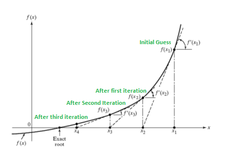
Suppose we have some function \( f : \mathbb{R} \mapsto \mathbb{R} \), and we wish to find a value of \(\theta\) so that \( f(\theta) = 0 \). Here, \(\theta \in \mathbb{R}\) is a real number. Newton's method performs the following update:

\[ \theta := \theta - \frac{f(\theta)}{f'(\theta)}. \]

This method has a natural interpretation in which we can think of it as approximating the function \( f \) via a linear function that is tangent to \( f \) at the current guess \(\theta\), solving for where that linear function equals to zero, and letting the next guess for \(\theta\) be where that linear function is zero.

Newton's Method

Definition (Newton-Raphson Method)

Newton's method gives a way of getting to \( f(\theta) = 0 \). What if we want to use it to maximize some function \(\ell\)? The maxima of \(\ell\) correspond to points where its first derivative \(\ell'(\theta)\) is zero. So, by letting \( f(\theta) = \ell'(\theta) \), we can use the same algorithm to maximize \(\ell\), and we obtain the update rule:

\[ \theta := \theta - \frac{\ell'(\theta)}{\ell''(\theta)}. \]

Lastly, in our logistic regression setting, \(\theta\) is vector-valued, so we need to generalize Newton's method to this setting. The generalization of Newton's method to this multidimensional setting (also called the Newton-Raphson Method) is given by

\[ \theta := \theta - H^{-1} \nabla_{\theta} \ell(\theta). \]

Note (Limitation of Newton's Method)

Newton's Method always bring us to the nearest stationary point instead of the global extreme, whereas GD does not have this limitation.