Neural Network Architectures

Note (Naming Conventions)

Notice that when we say N-layer neural network, we do not count the input layer. Therefore, a single-layer neural network describes a network with no hidden layers (input directly mapped to output). You may also hear these networks interchangeably referred to as “Artificial Neural Networks” (ANN) or “Multi-Layer Perceptrons” (MLP).

Representational Power

One way to look at Neural Networks with fully-connected layers is that they define a family of functions that are parameterized by the weights of the network. A natural question that arises is: Are there functions that cannot be modeled with a Neural Network?

Lemma (Representational Power of Neuron Network)

Given any continuous function \(f(x)\) and some \(\epsilon>0\), there exists a Neural Network \(g(x)\) with one hidden layer (with a reasonable choice of non-linearity, e.g. sigmoid) such that \(\forall x,\left| f(x)−g(x) \right| < \epsilon\). In other words, the neural network can approximate any continuous function.

Note (Why Not One Hidden Layer?)

If one hidden layer suffices to approximate any function, why use more layers and go deeper? The answer is that the fact that a two-layer Neural Network is a universal approximator is, while mathematically cute, a relatively weak and useless statement in practice. The fact that deeper networks (with multiple hidden layers) can work better than a single-hidden-layer networks is an empirical observation, despite the fact that their representational power is equal.

Note (More Layers or Not?)

In practice it is often the case that 3-layer neural networks will outperform 2-layer nets, but going even deeper (4,5,6-layer) rarely helps much more. This is in stark contrast to Convolutional Networks, where depth has been found to be an extremely important component for a good recognition system (e.g. on order of 10 learnable layers). One argument for this observation is that images contain hierarchical structure (e.g. faces are made up of eyes, which are made up of edges, etc.), so several layers of processing make intuitive sense for this data domain.

Important Note (Setting Number of Layers and Their Sizes)

How do we decide on what architecture to use when faced with a practical problem? First, note that as we increase the size and number of layers in a Neural Network, neurons can collaborate to express many more different functions.

A Binary Classification Problem

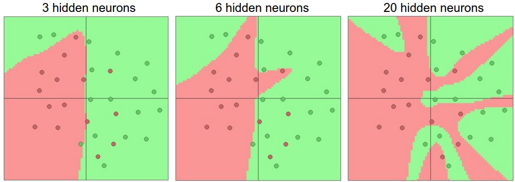
However, overfitting occurs if the NN has too much capability. But this does not mean we should choose a smaller model to avoid overfitting - there are many other preferred ways to prevent overfitting in Neural Networks such as L2 regularization, dropout, input noise. In practice, it is always better to use these methods to control overfitting instead of the number of neurons. The regularization strength is the preferred way to control the overfitting of a neural network. We can look at the results achieved by three different settings:

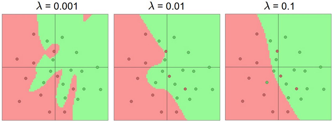
Changing the regularization strength makes its final decision regions smoother with a higher regularization. You can play this here.

Data Preprocessing

There are three common forms of data preprocessing a data matrix X, where we will assume that X is of size [N x D] (N is the number of data, D is their dimensionality).

Strategy (Mean Subtraction)

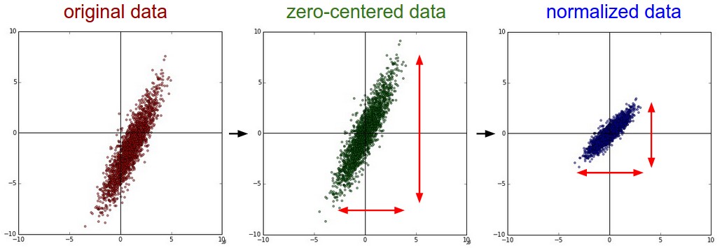
Mean subtraction is the most common form of preprocessing. It involves subtracting the mean across every individual feature in the data, and has the geometric interpretation of centering the cloud of data around the origin along every dimension. In numpy, this operation would be implemented as: X -= np.mean(X, axis=0). With images specifically, for convenience it can be common to subtract a single value from all pixels (e.g. X -= np.mean(X)), or to do so separately across the three color channels.

Strategy (Normalization)

Normalization refers to normalizing the data dimensions so that they are of approximately the same scale. There are two common ways of achieving this normalization. One is to divide each dimension by its standard deviation, once it has been zero-centered: X /= np.std(X, axis=0). Another form of this preprocessing normalizes each dimension so that the min and max along the dimension is -1 and 1 respectively. It only makes sense to apply this preprocessing if you have a reason to believe that different input features have different scales (or units), but they should be of approximately equal importance to the learning algorithm. In case of images, the relative scales of pixels are already approximately equal (and in range from 0 to 255), so it is not strictly necessary to perform this additional preprocessing step.

Common Data Preprocessing Pipeline

Strategy (PCA and Whitening)

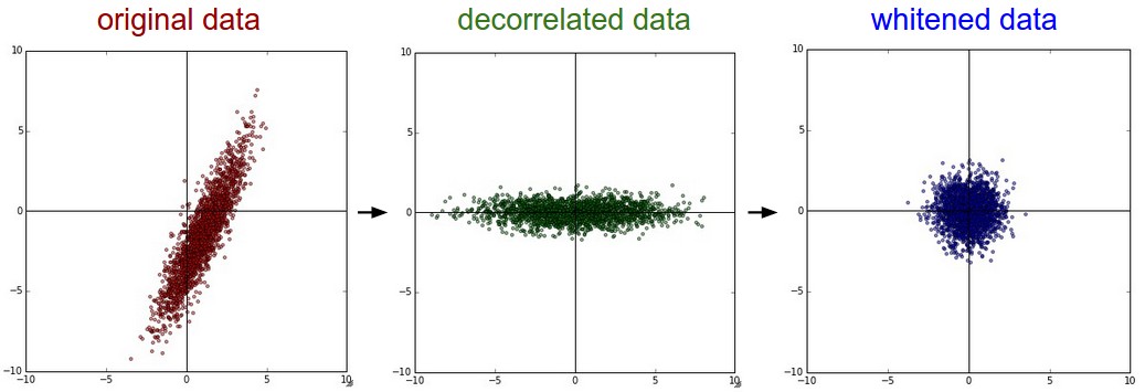
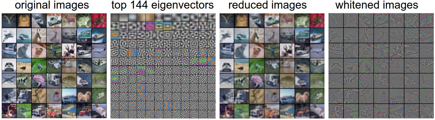
PCA and Whitening is another form of preprocessing. In this process, the data is first centered as described above. Then, we can compute the covariance matrix that tells us about the correlation structure in the data:

• PCA and Whitening

Example (Visualizing Whitened Images)

The training set of CIFAR-10 is of size 50,000 x 3072, where every image is stretched out into a 3072-dimensional row vector. We can then compute the [3072 x 3072] covariance matrix and compute its SVD decomposition (which can be relatively expensive). What do the computed eigenvectors look like visually? An image might help:

PCA / Whitening

Important Note (In Practice)

We mention PCA/Whitening in these notes for completeness, but these transformations are not used with Convolutional Networks. However, it is very important to zero-center the data, and it is common to see normalization of every pixel as well.

Warning (Only Preprocess Training Data)

Any preprocessing statistics (e.g. the data mean) must only be computed on the training data, and then applied to the validation / test data.

Weight Initialization

We have seen how to construct a Neural Network architecture, and how to preprocess the data. Before we can begin to train the network we have to initialize its parameters.

Warning (Pitfall: All Zero Initialization)

At the end of training, with a proper data normalization it is reasonable to assume that approximately half of the weights will be positive and half of them will be negative. We should not set all parameters to be 0 because if every neuron in the network computes the same output, then they will also all compute the same gradients during backpropagation and undergo the exact same parameter updates.

Strategy (Small Random Numbers Initialization)

It is common to initialize the weights of the neurons to small numbers and refer to doing so as symmetry breaking. The implementation for one weight matrix might look like W = 0.01* np.random.randn(D,H), where randn samples from a zero mean, unit standard deviation Gaussian.

Warning (Limitation of Small Random Numbers Initialization)

It’s not necessarily the case that smaller numbers will work strictly better. For example, a Neural Network layer that has very small weights will during backpropagation compute very small gradients on its data (since this gradient is proportional to the value of the weights). This could greatly diminish the “gradient signal” flowing backward through a network, and could become a concern for deep networks.

Strategy (Calibrating The Variances with \(\frac{1}{\sqrt{n}}\))

One problem with the above suggestion is that the distribution of the outputs from a randomly initialized neuron has a variance that grows with the number of inputs. It turns out that we can normalize the variance of each neuron’s output to 1 by scaling its weight vector by the square root of its fan-in (i.e. its number of inputs). That is, the recommended heuristic is to initialize each neuron’s weight vector as: w = np.random.randn(n) / sqrt(n), where n is the number of its inputs. This ensures that all neurons in the network initially have approximately the same output distribution and empirically improves the rate of convergence.

• Proof of this Strategy

Strategy (Sparse Initialization)

Another way to address the uncalibrated variances problem is to set all weight matrices to zero, but to break symmetry every neuron is randomly connected (with weights sampled from a small gaussian as above) to a fixed number of neurons below it. A typical number of neurons to connect to may be as small as 10.

Important Note (Initializing The Biases)

It is common to initialize the biases to be zero. For ReLU non-linearities, some people like to use small constant value such as 0.01 because this ensures that all ReLU units fire in the beginning and therefore obtain and propagate some gradient. However, it is not clear if this is useful and it is more common to simply use 0 bias initialization.

Important Note (In Practice)

The current recommendation is to use ReLU units and use the w = np.random.randn(n) * sqrt(2.0/n), as discussed in He et al..

Strategy (Batch Normalization)

A recently developed technique by Ioffe and Szegedy called Batch Normalization alleviates a lot of headaches with properly initializing neural networks by explicitly forcing the activations throughout a network to take on a unit gaussian distribution at the beginning of the training.

Regularization

There are several ways of controlling the capacity of Neural Networks to prevent overfitting:

Strategy (L2 Regularization)

For every weight \(w\) in the network, we add the term \(\frac{1}{2}\lambda w^2\) to the objective, where \(\lambda\) is the regularization strength.

Strategy (L1 Regularization)

For each weight \(w\) we add the term \(\lambda \left| w \right|\) to the objective.

Note (L2 v.s. L1)

In practice, if you are not concerned with explicit feature selection, L2 regularization can be expected to give superior performance over L1.

Strategy (Elastic Net Regularization)

Elastic net regularization is a combination of L1 & L2 regularization: \(\lambda_1 \left| w \right| + \lambda_2 w^2\).

Strategy (Max Norm Constraints)

Max norm put constraints to enforce an absolute upper bound on the magnitude of the weight vector for every neuron and use projected gradient descent to enforce the constraint. In practice, this corresponds to performing the parameter update as normal, and then enforcing the constraint by clamping the weight vector \(\vec{w}\) of every neuron to satisfy \(\|\vec{w}\|_2 < c\). Typical values of c are on orders of 3 or 4. Some people report improvements when using this form of regularization. One of its appealing properties is that network cannot "explode" even when the learning rates are set too high because the updates are always bounded.

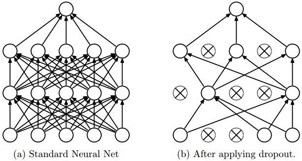
Strategy (Dropout)

Dropout is an extremely effective, simple and recently introduced regularization technique by Srivastava et al. in Dropout: A Simple Way to Prevent Neural Networks from Overfitting that complements the other methods (L1, L2, maxnorm). While training, dropout is implemented by only keeping a neuron active with some probability \(p\) (a hyperparameter), or setting it to zero otherwise.

Important Note (In Practice)

It is most common to use a single, global L2 regularization strength that is cross-validated. It is also common to combine this with dropout applied after all layers. The value of \(p=0.5\) is a reasonable default, but this can be tuned on validation data.

Important Note (Implementing Dropout)

def dropout_forward(x, dropout_param):
    """Forward pass for inverted dropout.

    Note that this is different from the vanilla version of dropout.
    Here, p is the probability of keeping a neuron output, as opposed to
    the probability of dropping a neuron output.
    See http://cs231n.github.io/neural-networks-2/#reg for more details.

    Inputs:
    - x: Input data, of any shape
    - dropout_param: A dictionary with the following keys:
    - p: Dropout parameter. We keep each neuron output with probability p.
    - mode: 'test' or 'train'. If the mode is train, then perform dropout;
        if the mode is test, then just return the input.
    - seed: Seed for the random number generator. Passing seed makes this
        function deterministic, which is needed for gradient checking but not
        in real networks.

    Outputs:
    - out: Array of the same shape as x.
    - cache: tuple (dropout_param, mask). In training mode, mask is the dropout
    mask that was used to multiply the input; in test mode, mask is None.
    """
    p, mode = dropout_param["p"], dropout_param["mode"]
    if "seed" in dropout_param:
        np.random.seed(dropout_param["seed"])

    mask = None
    out = None

    if mode == "train":
        mask = (np.random.rand(*x.shape) < p) / p
        out = x * mask

    elif mode == "test":
        out = x
        mask = None

    cache = (dropout_param, mask)
    out = out.astype(x.dtype, copy=False)

    return out, cache


def dropout_backward(dout, cache):
    """Backward pass for inverted dropout.

    Inputs:
    - dout: Upstream derivatives, of any shape
    - cache: (dropout_param, mask) from dropout_forward.
    """
    dropout_param, mask = cache
    mode = dropout_param["mode"]

    dx = None
    if mode == "train":
        dx = dout * mask

    elif mode == "test":
        dx = dout
    return dx

So far, we’ve discussed the static parts of a Neural Networks: how we can set up the network connectivity, the data, and the loss function. Now, we'll discuss the dynamics, or in other words, the process of learning the parameters and finding good hyperparameters.

Gradient Checks

Performing a gradient check is as simple as comparing the analytic gradient to the numerical gradient. In practice, the process is much more involved and error prone. Here are some tips, tricks, and issues to watch out for: (We discuss a lot of strategies. Non of them are trivial, however.)

Strategy (Gradient Checks: Use The Centered Formula)

The formula for the finite difference approximation when evaluating the numerical gradient looks as follows:

\[ \frac{df(x)}{dx} = \frac{f(x+h) - f(x)}{h} \quad (\text{bad, do not use}) \]

where \( h \) is a very small number, approximately 1e-5 or so. In practice, it turns out that it is much better to use the centered difference formula of the form:

\[ \frac{df(x)}{dx} = \frac{f(x+h) - f(x-h)}{2h} \quad (\text{use instead}) \]

This requires you to evaluate the loss function twice to check every single dimension of the gradient (so it is about 2 times as expensive), but the gradient approximation turns out to be much more precise. To see this, you can use Taylor expansion of \( f(x+h) \) and \( f(x-h) \) and verify that the first formula has an error on order of \( O(h) \), while the second formula only has error terms on order of \( O(h^2) \) (i.e. it is a second order approximation).

• Proof

Strategy (Gradient Checks: Use Relative Error for The Comparison)

How do we know if the two gradients are not compatible? We should not use the difference \( |f'_a - f'_n| \) and define the gradient check as failed if that difference is above a threshold. For example, consider the case where their difference is 1e-4. This seems like a very appropriate difference if the two gradients are about 1.0, but if the gradients were both on order of 1e-5 or lower, then we’d consider 1e-4 to be a huge difference and likely a failure. Hence, it is always more appropriate to consider the relative error:

\[ \frac{|f'_a - f'_n|}{\max(|f'_a|, |f'_n|)} \]

Notice that normally the relative error formula only includes one of the two terms (either one), but I prefer to max (or add) both to make it symmetric and to prevent dividing by zero in the case where one of the two is zero (which can often happen, especially with ReLUs). However, one must explicitly keep track of the case where both are zero and pass the gradient check in that edge case.

In practice:

• relative error > 1e-2 usually means the gradient is probably wrong
• 1e-2 > relative error > 1e-4 should make you feel uncomfortable
• 1e-4 > relative error is usually okay for objectives with kinks. But if there are no kinks (e.g. use of tanh nonlinearities and softmax), then 1e-4 is too high.
• 1e-7 and less you should be happy.

Note (Deeper The Network, Higher The Error)

Note that the deeper the network, the higher the relative errors will be. So if you are gradient checking the input data for a 10-layer network, a relative error of 1e-2 might be okay because the errors build up on the way. Conversely, an error of 1e-2 for a single differentiable function likely indicates incorrect gradient.

Warning (Use Double Precision)

A common pitfall is using single precision floating point to compute gradient check. It is often that case that you might get high relative errors (as high as 1e-2) even with a correct gradient implementation. In my experience I’ve sometimes seen my relative errors plummet from 1e-2 to 1e-8 by switching to double precision.

Strategy (Gradient Checks: Stick Around Active Range of Floating Point)

It's a good idea to read through “What Every Computer Scientist Should Know About Floating-Point Arithmetic”, as it may demystify your errors and enable you to write more careful code. For example, in neural nets it can be common to normalize the loss function over the batch. However, if your gradients per datapoint are very small, then additionally dividing them by the number of data points is starting to give very small numbers, which in turn will lead to more numerical issues. This is why I like to always print the raw numerical/analytic gradient, and make sure that the numbers you are comparing are not extremely small (e.g. roughly 1e-10 and smaller in absolute value is worrying). If they are you may want to temporarily scale your loss function up by a constant to bring them to a “nicer” range where floats are more dense - ideally on the order of 1.0, where your float exponent is 0.

Strategy (Gradient Checks: Kinks in The Objective)

One source of inaccuracy to be aware of during gradient checking is the problem of kinks. Kinks refer to non-differentiable parts of an objective function, introduced by functions such as ReLU (\(\max(0, x)\)), or the SVM loss, Maxout neurons, etc. Consider gradient checking the ReLU function at \( x = -1e6 \). Since \( x < 0 \), the analytic gradient at this point is exactly zero. However, the numerical gradient would suddenly compute a non-zero gradient because \( f(x+h) \) might cross over the kink (e.g. if \( h > 1e-6 \)) and introduce a non-zero contribution. You might think that this is a pathological case, but in fact this case can be very common. For example, an SVM for CIFAR-10 contains up to 450,000 \(\max(0, x)\) terms because there are 50,000 examples and each example yields 9 terms to the objective. Moreover, a Neural Network with an SVM classifier will contain many more kinks due to ReLUs.

Note that it is possible to know if a kink was crossed in the evaluation of the loss. This can be done by keeping track of the identities of all “winners” in a function of form \(\max(x, y)\); That is, was \( x \) or \( y \) higher during the forward pass. If the identity of at least one winner changes when evaluating \( f(x+h) \) and then \( f(x-h) \), then a kink was crossed and the numerical gradient will not be exact.

Strategy (Gradient Checks: Use Only Few Datapoints)

One fix to the above problem of kinks is to use fewer datapoints, since loss functions that contain kinks (e.g. due to use of ReLUs or margin losses etc.) will have fewer kinks with fewer datapoints, so it is less likely for you to cross one when you perform the finite different approximation. Moreover, if your gradcheck for only ~2 or 3 datapoints then you would almost certainly gradcheck for an entire batch. Using very few datapoints also makes your gradient check faster and more efficient.

Strategy (Gradient Checks: Be Careful with The Step Size \( h \))

It is not necessarily the case that smaller is better, because when \( h \) is much smaller, you may start running into numerical precision problems. Sometimes when the gradient doesn’t check, it is possible that you change \( h \) to be 1e-4 or 1e-6 and suddenly the gradient will be correct. This wikipedia article contains a chart that plots the value of \( h \) on the x-axis and the numerical gradient error on the y-axis.

Strategy (Gradient Checks: Gradcheck During a “Characteristic” Mode of Operation)

It is important to realize that a gradient check is performed at a particular (and usually random), single point in the space of parameters. Even if the gradient check succeeds at that point, it is not immediately certain that the gradient is correctly implemented globally. Additionally, a random initialization might not be the most “characteristic” point in the space of parameters and may in fact introduce pathological situations where the gradient seems to be correctly implemented but isn’t. For instance, an SVM with very small weight initialization will assign almost exactly zero scores to all datapoints and the gradients will exhibit a particular pattern across all datapoints. An incorrect implementation of the gradient could still produce this pattern and not generalize to a more characteristic mode of operation where some scores are larger than others. Therefore, to be safe it is best to use a short burn-in time during which the network is allowed to learn and perform the gradient check after the loss starts to go down. The danger of performing it at the first iteration is that this could introduce pathological edge cases and mask an incorrect implementation of the gradient.

Strategy (Gradient Checks: Don’t Let The Regularization Overwhelm The Data)

It is often the case that a loss function is a sum of the data loss and the regularization loss (e.g. L2 penalty on weights). One danger to be aware of is that the regularization loss may overwhelm the data loss, in which case the gradients will be primarily coming from the regularization term (which usually has a much simpler gradient expression). This can mask an incorrect implementation of the data loss gradient. Therefore, it is recommended to turn off regularization and check the data loss alone first, and then the regularization term second and independently. One way to perform the latter is to hack the code to remove the data loss contribution. Another way is to increase the regularization strength so as to ensure that its effect is non-negligible in the gradient check, and that an incorrect implementation would be spotted.

Strategy (Gradient Checks: Remember to Turn off Dropout/Augmentations)

When performing gradient check, remember to turn off any non-deterministic effects in the network, such as dropout, random data augmentations, etc. Otherwise, these can clearly introduce huge errors when estimating the numerical gradient. The downside of turning off these effects is that you wouldn’t be gradient checking them (e.g. it might be that dropout isn’t backpropagated correctly). Therefore, a better solution might be to force a particular random seed before evaluating both \( f(x+h) \) and \( f(x-h) \), and when evaluating the analytic gradient.

Strategy (Gradient Checks: Check Only Few Dimensions)

In practice the gradients can have sizes of million parameters. In these cases it is only practical to check some of the dimensions of the gradient and assume that the others are correct. Be careful: One issue to be careful with is to make sure to gradient check a few dimensions for every separate parameter. In some applications, people combine the parameters into a single large parameter vector for convenience. In these cases, for example, the biases could only take up a tiny number of parameters from the whole vector, so it is important to not sample at random but to take this into account and check that all parameters receive the correct gradients.

Important Note (Gradient Checks in Code)

def eval_numerical_gradient(f, x, verbose=True, h=0.00001):
    """
    a naive implementation of numerical gradient of f at x
    - f should be a function that takes a single argument
    - x is the point (numpy array) to evaluate the gradient at
    """

    fx = f(x)  # evaluate function value at original point
    grad = np.zeros_like(x)
    # iterate over all indexes in x
    it = np.nditer(x, flags=["multi_index"], op_flags=["readwrite"])
    while not it.finished:

        # evaluate function at x+h
        ix = it.multi_index
        oldval = x[ix]
        x[ix] = oldval + h  # increment by h
        fxph = f(x)  # evalute f(x + h)
        x[ix] = oldval - h
        fxmh = f(x)  # evaluate f(x - h)
        x[ix] = oldval  # restore

        # compute the partial derivative with centered formula
        grad[ix] = (fxph - fxmh) / (2 * h)  # the slope
        if verbose:
            print(ix, grad[ix])
        it.iternext()  # step to next dimension

    return grad

def eval_numerical_gradient_array(f, x, df, h=1e-5):
    """
    Evaluate a numeric gradient for a function that accepts a numpy
    array and returns a numpy array.
    """
    grad = np.zeros_like(x)
    it = np.nditer(x, flags=["multi_index"], op_flags=["readwrite"])
    while not it.finished:
        ix = it.multi_index

        oldval = x[ix]
        x[ix] = oldval + h
        pos = f(x).copy()
        x[ix] = oldval - h
        neg = f(x).copy()
        x[ix] = oldval

        grad[ix] = np.sum((pos - neg) * df) / (2 * h)
        it.iternext()
    return grad

def eval_numerical_gradient_blobs(f, inputs, output, h=1e-5):
    """
    Compute numeric gradients for a function that operates on input
    and output blobs.

    We assume that f accepts several input blobs as arguments, followed by a
    blob where outputs will be written. For example, f might be called like:

    f(x, w, out)

    where x and w are input Blobs, and the result of f will be written to out.

    Inputs:
    - f: function
    - inputs: tuple of input blobs
    - output: output blob
    - h: step size
    """
    numeric_diffs = []
    for input_blob in inputs:
        diff = np.zeros_like(input_blob.diffs)
        it = np.nditer(input_blob.vals, flags=["multi_index"], op_flags=["readwrite"])
        while not it.finished:
            idx = it.multi_index
            orig = input_blob.vals[idx]

            input_blob.vals[idx] = orig + h
            f(*(inputs + (output,)))
            pos = np.copy(output.vals)
            input_blob.vals[idx] = orig - h
            f(*(inputs + (output,)))
            neg = np.copy(output.vals)
            input_blob.vals[idx] = orig

            diff[idx] = np.sum((pos - neg) * output.diffs) / (2.0 * h)

            it.iternext()
        numeric_diffs.append(diff)
    return numeric_diffs

def eval_numerical_gradient_net(net, inputs, output, h=1e-5):
    return eval_numerical_gradient_blobs(
        lambda *args: net.forward(), inputs, output, h=h
    )

def grad_check_sparse(f, x, analytic_grad, num_checks=10, h=1e-5):
    """
    sample a few random elements and only return numerical
    in this dimensions.
    """

    for i in range(num_checks):
        ix = tuple([randrange(m) for m in x.shape])

        oldval = x[ix]
        x[ix] = oldval + h  # increment by h
        fxph = f(x)  # evaluate f(x + h)
        x[ix] = oldval - h  # increment by h
        fxmh = f(x)  # evaluate f(x - h)
        x[ix] = oldval  # reset

        grad_numerical = (fxph - fxmh) / (2 * h)
        grad_analytic = analytic_grad[ix]
        rel_error = abs(grad_numerical - grad_analytic) / (
            abs(grad_numerical) + abs(grad_analytic)
        )
        print(
            "numerical: %f analytic: %f, relative error: %e"
            % (grad_numerical, grad_analytic, rel_error)
        )

Before Learning: Sanity Checks Tips/Tricks

Here are a few sanity checks you might consider running before you plunge into expensive optimization:

Strategy (Look for Correct Loss at Chance Performance)

Make sure you’re getting the loss you expect when you initialize with small parameters. It’s best to first check the data loss alone (so set regularization strength to zero). For example, for CIFAR-10 with a Softmax classifier we would expect the initial loss to be 2.302, because we expect a diffuse probability of 0.1 for each class (since there are 10 classes), and Softmax loss is the negative log probability of the correct class so: -ln(0.1) = 2.302. For The Weston Watkins SVM, we expect all desired margins to be violated (since all scores are approximately zero), and hence expect a loss of 9 (since margin is 1 for each wrong class). If you’re not seeing these losses there might be issue with initialization.

Note (Second Sanity Check)

As a second sanity check, increasing the regularization strength should increase the loss.

Strategy (Overfit a Tiny Subset of Data)

Lastly and most importantly, before training on the full dataset try to train on a tiny portion (e.g. 20 examples) of your data and make sure you can achieve zero cost. For this experiment it’s also best to set regularization to zero, otherwise this can prevent you from getting zero cost. Unless you pass this sanity check with a small dataset it is not worth proceeding to the full dataset. Note that it may happen that you can overfit very small dataset but still have an incorrect implementation. For instance, if your datapoints’ features are random due to some bug, then it will be possible to overfit your small training set but you will never notice any generalization when you fold it your full dataset.

Babysitting The Learning Process

There are multiple useful quantities you should monitor during training of a neural network. These plots are the window into the training process and should be utilized to get intuitions about different hyperparameter settings and how they should be changed for more efficient learning.

The x-axis of the plots below are always in units of epochs, which measure how many times every example has been seen during training in expectation (e.g. one epoch means that every example has been seen once). It is preferable to track epochs rather than iterations since the number of iterations depends on the arbitrary setting of batch size.

Important Note (Tracking Loss Function)

The first quantity that is useful to track during training is the loss, as it is evaluated on the individual batches during the forward pass. Below is a cartoon diagram showing the loss over time, and especially what the shape might tell you about the learning rate:

Effects of Different Learning Rates

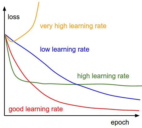
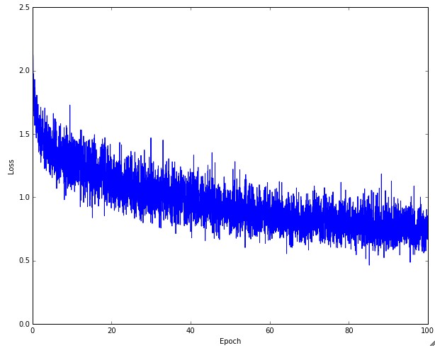
The amount of “wiggle” in the loss is related to the batch size. When the batch size is 1, the wiggle will be relatively high. When the batch size is the full dataset, the wiggle will be minimal because every gradient update should be improving the loss function monotonically (unless the learning rate is set too high).

Typical Loss Function over Time

Some people prefer to plot their loss functions in the log domain. Since learning progress generally takes an exponential form shape, the plot appears as a slightly more interpretable straight line, rather than a hockey stick. Additionally, if multiple cross-validated models are plotted on the same loss graph, the differences between them become more apparent.

Sometimes loss functions can look funny: LossFunctions

Important Note (Interpreting Train/Val Accuracy)

The second important quantity to track while training a classifier is the validation/training accuracy. This plot can give you valuable insights into the amount of overfitting in your model:

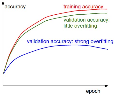
The gap between the training and validation accuracy indicates the amount of overfitting. Two possible cases are shown in the diagram on the left. The blue validation error curve shows very small validation accuracy compared to the training accuracy, indicating strong overfitting (note, it's possible for the validation accuracy to even start to go down after some point). When you see this in practice you probably want to increase regularization (stronger L2 weight penalty, more dropout, etc.) or collect more data. The other possible case is when the validation accuracy tracks the training accuracy fairly well. This case indicates that your model capacity is not high enough: make the model larger by increasing the number of parameters.

Important Note (Tracking Ratio of Weights: Updates)

The last quantity you might want to track is the ratio of the update magnitudes to the value magnitudes. Note: updates, not the raw gradients (e.g. in vanilla sgd this would be the gradient multiplied by the learning rate). You might want to evaluate and track this ratio for every set of parameters independently. A rough heuristic is that this ratio should be somewhere around 1e-3. If it is lower than this then the learning rate might be too low. If it is higher then the learning rate is likely too high. Here is a specific example:

# assume parameter vector W and its gradient vector dW
param_scale = np.linalg.norm(W.ravel())
update = -learning_rate*dW # simple SGD update
update_scale = np.linalg.norm(update.ravel())
W += update # the actual update
print update_scale / param_scale # want ~1e-3

Instead of tracking the min or the max, some people prefer to compute and track the norm of the gradients and their updates instead. These metrics are usually correlated and often give approximately the same results.

Important Note (Activation / Gradient Distributions Per Layer)

An incorrect initialization can slow down or even completely stall the learning process. Luckily, this issue can be diagnosed relatively easily. One way to do so is to plot activation/gradient histograms for all layers of the network. Intuitively, it is not a good sign to see any strange distributions - e.g. with tanh neurons we would like to see a distribution of neuron activations between the full range of [-1,1], instead of seeing all neurons outputting zero, or all neurons being completely saturated at either -1 or 1.

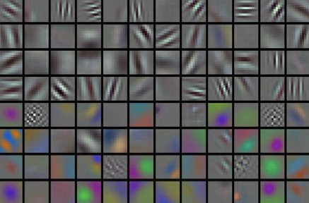
Strategy (First-layer Visualizations)

When one is working with image pixels it can be helpful and satisfying to plot the first-layer features visually:

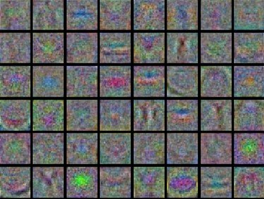
Left: Noisy features indicate could be a symptom: Unconverged network, improperly set learning rate, very low weight regularization penalty.

Right: Nice, smooth, clean and diverse features are a good indication that the training is proceeding well.

Parameter Updates

Once the analytic gradient is computed with backpropagation, the gradients are used to perform a parameter update. There are several approaches for performing the update, which we discuss next.

We note that optimization for deep networks is currently a very active area of research. In this section we highlight some established and common techniques you may see in practice and briefly describe their intuition.

Algorithm (Vanilla Update)

The Vanilla update is the simplest form of update: change the parameters along the negative gradient direction (since the gradient indicates the direction of increase, but we usually wish to minimize a loss function). Assuming a vector of parameters x and the gradient dx, the simplest update has the form:

# Vanilla update
x += - learning_rate * dx

where learning_rate is a hyperparameter. When evaluated on the full dataset, and when the learning rate is low enough, this is guaranteed to make non-negative progress on the loss function.

Algorithm (SGD)

Important Note (Implementing sgd)

def update(w, dw, config=None):
    """
    Inputs:
    - w: A numpy array giving the current weights.
    - dw: A numpy array of the same shape as w giving the gradient of the
        loss with respect to w.
    - config: A dictionary containing hyperparameter values such as learning
        rate, momentum, etc. If the update rule requires caching values over many
        iterations, then config will also hold these cached values.

    Returns:
    - next_w: The next point after the update.
    - config: The config dictionary to be passed to the next iteration of the
        update rule.

    NOTE: For most update rules, the default learning rate will probably not
    perform well; however the default values of the other hyperparameters should
    work well for a variety of different problems.

    For efficiency, update rules may perform in-place updates, mutating w and
    setting next_w equal to w.
    """

def sgd(w, dw, config=None):
    """
    Performs vanilla stochastic gradient descent.

    config format:
    - learning_rate: Scalar learning rate.
    """
    if config is None:
        config = {}
    config.setdefault("learning_rate", 1e-2)

    w -= config["learning_rate"] * dw
    return w, config

Algorithm (Momentum Update)

Important Note (Implementing Momentum (with sgd))

def sgd_momentum(w, dw, config=None):
    """
    Performs stochastic gradient descent with momentum.

    config format:
    - learning_rate: Scalar learning rate.
    - momentum: Scalar between 0 and 1 giving the momentum value.
    Setting momentum = 0 reduces to sgd.
    - velocity: A numpy array of the same shape as w and dw used to store a
    moving average of the gradients.
    """
    if config is None:
        config = {}
    config.setdefault("learning_rate", 1e-2)
    config.setdefault("momentum", 0.9)
    v = config.get("velocity", np.zeros_like(w))

    next_w = None

    v = config["momentum"] * v - config["learning_rate"] * dw
    next_w = w + v

    config["velocity"] = v

    return next_w, config

Algorithm (rmsprop)

Important Note (Implementing rmsprop)

def rmsprop(w, dw, config=None):
"""
Uses the RMSProp update rule, which uses a moving average of squared
gradient values to set adaptive per-parameter learning rates.

config format:
- learning_rate: Scalar learning rate.
- decay_rate: Scalar between 0 and 1 giving the decay rate for the squared
  gradient cache.
- epsilon: Small scalar used for smoothing to avoid dividing by zero.
- cache: Moving average of second moments of gradients.
"""
if config is None:
    config = {}
config.setdefault("learning_rate", 1e-2)
config.setdefault("decay_rate", 0.99)
config.setdefault("epsilon", 1e-8)
config.setdefault("cache", np.zeros_like(w))

next_w = None

config['cache'] = config['decay_rate'] * config['cache'] + (1 - config['decay_rate']) * (dw ** 2)
next_w = w - config['learning_rate'] / np.sqrt(config['cache'] + config['epsilon']) * dw

return next_w, config

Algorithm (Adam)

Important Note (Implementing Adam)

def adam(w, dw, config=None):
    """
    Uses the Adam update rule, which incorporates moving averages of both the
    gradient and its square and a bias correction term.

    config format:
    - learning_rate: Scalar learning rate.
    - beta1: Decay rate for moving average of first moment of gradient.
    - beta2: Decay rate for moving average of second moment of gradient.
    - epsilon: Small scalar used for smoothing to avoid dividing by zero.
    - m: Moving average of gradient.
    - v: Moving average of squared gradient.
    - t: Iteration number.
    """
    if config is None:
        config = {}
    config.setdefault("learning_rate", 1e-3)
    config.setdefault("beta1", 0.9)
    config.setdefault("beta2", 0.999)
    config.setdefault("epsilon", 1e-8)
    config.setdefault("m", np.zeros_like(w))
    config.setdefault("v", np.zeros_like(w))
    config.setdefault("t", 0)

    next_w = None

    keys = ["learning_rate", "beta1", "beta2", "epsilon", "m", "v", "t"]
    lr, beta1, beta2, epsilon, m, v, t = (config.get(key) for key in keys)

    t += 1
    m = beta1 * m + (1 - beta1) * dw
    mt = m / (1 - beta1 ** t)
    v = beta2 * v + (1 - beta2) * (dw**2)
    vt = v / (1 - beta2 ** t)
    next_w = w - lr * mt / (np.sqrt(vt) + epsilon)

    config['t'] = t
    config['m'] = m
    config['v'] = v

    return next_w, config

Hyperparameter Optimization

Evaluation

Strategy (Model Ensembles)

In practice, one reliable approach to improving the performance of Neural Networks by a few percent is to train multiple independent models, and at test time average their predictions. As the number of models in the ensemble increases, the performance typically monotonically improves (though with diminishing returns). Moreover, the improvements are more dramatic with higher model variety in the ensemble. There are a few approaches to forming an ensemble:

• Same model, different initializations. Use cross-validation to determine the best hyperparameters, then train multiple models with the best set of hyperparameters but with different random initialization. The danger with this approach is that the variety is only due to initialization.
• Top models discovered during cross-validation. Use cross-validation to determine the best hyperparameters, then pick the top few (e.g. 10) models to form the ensemble. This improves the variety of the ensemble but has the danger of including suboptimal models. In practice, this can be easier to perform since it doesn’t require additional retraining of models after cross-validation.
• Different checkpoints of a single model. If training is very expensive, some people have had limited success in taking different checkpoints of a single network over time (for example after every epoch) and using those to form an ensemble. Clearly, this suffers from some lack of variety, but can still work reasonably well in practice. The advantage of this approach is that it is very cheap.
• Running average of parameters during training. Related to the last point, a cheap way of almost always getting an extra percent or two of performance is to maintain a second copy of the network’s weights in memory that maintains an exponentially decaying sum of previous weights during training. This way you’re averaging the state of the network over last several iterations. You will find that this “smoothed” version of the network almost always achieves better validation error. The rough intuition to have in mind is that the objective is bowl-shaped and your network is jumping around the mode, so the average has a higher chance of being somewhere nearer the mode.

One disadvantage of model ensembles is that they take longer to evaluate on test examples. An interested reader may find the recent work from Geoff Hinton on “Dark Knowledge” inspiring, where the idea is to “distill” a good ensemble back to a single model by incorporating the ensemble log likelihoods into a modified objective.